Wiener process regression in LazyPPL
Extensions and imports for this Literate Haskell file
{-# LANGUAGE CPP #-}
module WienerDemo where
import LazyPPL
import LazyPPL.Distributions
import LazyPPL.Distributions.GP (wiener)

import Data.List
import Data.Map (empty,lookup,insert,size,keys)
import Control.Monad
import Numeric.Log (Log(Exp))
import Data.IORef
import System.IO.Unsafeimport Graphics.Matplotlib hiding (density)We can define a random function wiener :: Prob(Double -> Double) which describes a Wiener process. This requires an infinite number of random choices, first because it is defined for arbitrarily large x, but also it needs an infinite number of random choices in each finite interval, because it is no-where differentiable. This is all dealt with using laziness. We can’t plot this unbounded, undifferentiable function precisely, but when we plot it with a fixed resolution and viewport, the necessary finite random choices are triggered. 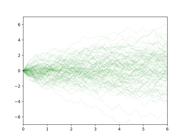
(Plotting code)
plotWienerPrior =
  do
    fws <- mh 1 $ sample wiener
    let xys = map (\f -> map (\x -> (x,f x)) [0,0.1..6]) $ map fst $ take 100 $ fws
plotCoords "images/wiener-prior.svg" [] xys (-7) 7 0.2dataset :: [(Double, Double)]
dataset = [(0,0.6), (1, 0.7), (2,1.2), (3,3.2), (4,6.8), (5, 8.2), (6,8.4)]g plus a random start point a. (Note that we are treating this g as a function like any other. And we could also have built this model with the second-order regress function from the other regression examples.)
example :: Meas (Double -> Double)
example = do g <- sample wiener
             a <- sample $ normal 0 3
             let f x = a + 2 * (g x)
             forM_ dataset (\(x,y) -> scoreLog $ Exp $ normalLogPdf (f x) 0.3 y)
return fplotWienerRegression =
do
fws <- mh 0.1 example
let xys = map (\f -> map (\x -> (x,f x)) [0,0.1..6]) $ map fst $ take 100 $ every 1000 $ drop 10000 $ fws
plotCoords "images/wiener-reg.svg" dataset xys (-2) 10 0.1Wiener-process regression
Ready.
- 95% predictive interval
- log-likelihood low high
- Observations
Numerical results
Scroll within the table for more values.
Ready.
- log-likelihood low high
- Observations
Numerical results
Scroll within the table for more values.
Ready.
- log-likelihood low high
- Observations
Numerical results
Scroll within the table for more values.
Ready.
- Posterior programs (lines)
- Observations
Numerical results
Scroll within the table for more values.
Ready.
- log-likelihood low high
- Observations
Numerical results
Scroll within the table for more values.

Jump diffusion compositionally
Recall the splice function splice :: Prob [Double] -> Prob (Double -> Double) -> Prob (Double -> Double) from the linear regression example, which pieces together draws from a random function using a point process. We can immediately apply this to the Wiener process, to get a jump diffusion process.
Recalling splice function and Poisson point process
splice :: Prob [Double] -> Prob (Double -> Double) -> Prob (Double -> Double)
splice pointProcess randomFun =
  do
    xs <- pointProcess
    fs <- mapM (const randomFun) xs
    default_f <- randomFun
    let h :: [(Double, Double -> Double)] -> Double -> Double
        h [] x = default_f x
        h ((a, f) : xfs) x | x <= a = f x
        h ((a, f) : xfs) x | x > a = h xfs x
    return (h (zip xs fs))

poissonPP :: Double -> Double -> Prob [Double]
poissonPP lower rate =
  do
    step <- exponential rate
    let x = lower + step
    xs <- poissonPP x rate
    return (x : xs)

regress :: Double -> Prob (a -> Double) -> [(a, Double)] -> Meas (a -> Double)
regress sigma prior dataset =
  do
    f <- sample prior
    forM_ dataset (\(x, y) -> scoreLog $ Exp $ normalLogPdf (f x) sigma y)
return fjump :: Prob (Double -> Double)
jump = let p = do f <- wiener
a <- normal 0 3
return $ \x -> a + f x
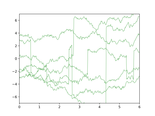
in splice (poissonPP 0 0.2) pHere are six samples from this distribution.
(Plotting code)
plotJumpPrior =
  do
    fws <- mh 1 $ sample jump
    let xys = map (\f -> map (\x -> (x,f x)) [0,0.02..6]) $ map fst $ take 6 $ fws
plotCoords "images/wiener-jump-prior.svg" [] xys (-7) 7 1datasetB :: [(Double, Double)]
datasetB = [(0,0.6), (1, 0.7), (2,8.2), (3,9.1), (4,3.2), (5,4.9), (6,2.9)]plotJumpRegression =
do
fws <- mhirreducible 0.2 0.1 (regress 0.3 jump datasetB)
let xys = map (\f -> map (\x -> (x,f x)) [0,0.02..6]) $ map fst $ take 100 $ every 1000 $ drop 300000 $ fws
plotCoords "images/wiener-jump-reg.svg" datasetB xys (-2) 10 0.1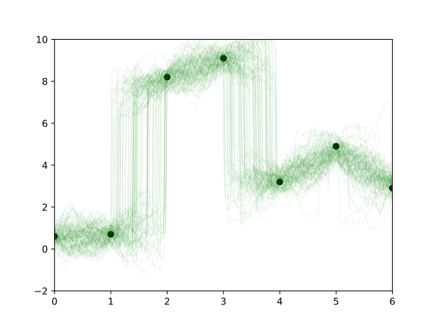
Graphing routines
plotCoords :: String -> [(Double,Double)] -> [[(Double,Double)]] -> Double -> Double -> Double -> IO ()
plotCoords filename dataset xyss ymin ymax alpha =
    do  putStrLn $ "Plotting " ++ filename ++ "..."
        file filename $ foldl (\a xys -> a % plot (map fst xys) (map snd xys) @@ [o1 "go-", o2 "linewidth" (0.5 :: Double), o2 "alpha" alpha, o2 "ms" (0 :: Int)]) (scatter (map fst dataset) (map snd dataset) @@ [o2 "c" "black"] % xlim (0 :: Int) (6 :: Int) % ylim ymin ymax) xyss
        putStrLn "Done."
        return ()


main :: IO ()
main = do { plotWienerPrior ; plotWienerRegression ; plotJumpPrior ; plotJumpRegression }