Probabilistic programming with graphs, and graph inference
We discuss probabilistic programming with graphs and graph inference. The key idea is to work with an abstract interface with an abstract Vertex of vertices, a probability distribution new on Vertex, and an edge relation edge :: Vertex -> Vertex -> Bool.
This file is a literate Haskell file, see the readme file for details.
The code uses the LazyPPL library for Haskell which provides an affine probability monad Prob and Metropolis-Hastings inference methods. Similar code would work in many other probabilistic programming languages; the advantage of LazyPPL is that it has types, supports memoization, and has an explicitly separate affine monad Prob.
Extensions and imports for this Literate Haskell file
{-# LANGUAGE CPP #-}
{-# LANGUAGE FlexibleInstances #-}
{-# LANGUAGE MultiParamTypeClasses #-}
{-# LANGUAGE FunctionalDependencies #-}
{-# LANGUAGE UndecidableInstances #-}
{-# LANGUAGE ScopedTypeVariables #-}
{-# LANGUAGE ExtendedDefaultRules #-}
module GraphDemo where
import LazyPPL
import LazyPPL.Distributions
import LazyPPL.Distributions.Memoization
import Control.Monad
import Data.List
import Data.Maybe
import Numeric.Log (Log(Exp))import Graphics.Matplotlib
import Graphics.Matplotlib hiding (density)instance MonadMemo Prob Double where
memoize = generalmemoizeIntro: graph inference problem
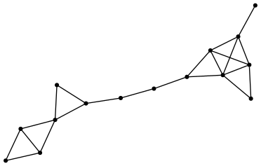
For an example inference problem, consider the following graph, which we call test. We will ask, which kinds of vertices and distribution on vertices likely generated it?
Code for adjacency matrix
test :: [[Bool]]
test = map (map $ \x -> x==1)
 [[0, 1, 1, 1, 0, 0, 0, 0, 0, 0, 0, 0, 0, 0, 0],
  [1, 0, 1, 1, 0, 0, 0, 0, 0, 0, 0, 0, 0, 0, 0],
  [1, 1, 0, 0, 0, 0, 0, 0, 0, 0, 0, 0, 0, 0, 0],
  [1, 1, 0, 0, 1, 1, 0, 0, 0, 0, 0, 0, 0, 0, 0],
  [0, 0, 0, 1, 0, 1, 1, 0, 0, 0, 0, 0, 0, 0, 0],
  [0, 0, 0, 1, 1, 0, 0, 0, 0, 0, 0, 0, 0, 0, 0],
  [0, 0, 0, 0, 1, 0, 0, 1, 0, 0, 0, 0, 0, 0, 0],
  [0, 0, 0, 0, 0, 0, 1, 0, 1, 0, 0, 0, 0, 0, 0],
  [0, 0, 0, 0, 0, 0, 0, 1, 0, 1, 1, 0, 0, 0, 0],
  [0, 0, 0, 0, 0, 0, 0, 0, 1, 0, 1, 1, 1, 1, 0],
  [0, 0, 0, 0, 0, 0, 0, 0, 1, 1, 0, 1, 1, 0, 0],
  [0, 0, 0, 0, 0, 0, 0, 0, 0, 1, 1, 0, 1, 1, 0],
  [0, 0, 0, 0, 0, 0, 0, 0, 0, 1, 1, 1, 0, 0, 1],
  [0, 0, 0, 0, 0, 0, 0, 0, 0, 1, 0, 1, 0, 0, 0],
[0, 0, 0, 0, 0, 0, 0, 0, 0, 0, 0, 0, 1, 0, 0]]showTestData = do
putStrLn "Generating graph-data.dot"
writeFile "graph-data.dot" $ graphToDot test
-- Convert the dot file to an svg using GraphViz, e.g. via
-- https://dreampuf.github.io/GraphvizOnlineAs we will show, we can, for example, infer some parameters to see whether it arises as a geometric graph, such as the following, or as an Erdős-Rényi graph, and so on.
Basics of the graph interface
We define a type class that describes our interface for random graphs, that include a parameterp, a type v of vertices, and new and edge functions.
class Show v => RandomGraph p v | p -> v where
  new :: p -> Prob v
  edge :: p -> v -> v -> Bool
Example random graph: geometric
The first kind of instance of this type class is a geometric graph on a sphere, parameterized by a dimension d :: Int and distance theta :: Double. Vertices are uniformly distributed on the sphere, and there is an edge between two vertices if their angle is less than theta.
data SphGrph = SG Int Double -- Graph parameters with dimension and distance
data SphVert = SV [Double]   -- Vertices are coordinates

instance Show SphVert where
  show (SV (x:y:xs)) = show x ++ "," ++ show (SV (y:xs))
  show (SV (x:[])) = show x

instance RandomGraph SphGrph SphVert where
  new (SG d theta) =
   do
     -- sample d-dimensional isotropic normal vectors
     xs <- replicateM d $ normal 0 1
     -- compute the length
     let r = sqrt $ sum $ map (^ 2) xs
     -- normalize, to get something on the sphere
     return $ SV $ map (/ r) xs
  edge (SG d theta) (SV xs) (SV ys) =
   theta > acos (max (-1) (min 1 (sum (zipWith (*) xs ys))))
Here, we have encoded the -sphere using -dimensional Euclidean coordinates. We are generating the points uniformly, by normalizing coordinates from a d-variate normal distribution. (Note that in Haskell this implementation detail could be hidden, by putting the implementation in a separate file and not exporting the SV constructor.)
Example random graph: graphons
Another way of specifying a random graph is by a graphon, which is a function .data Graphon = Graphon (Double -> Double -> Double)
data GraphonVertex = GV Double (Double->Bool)
instance Show GraphonVertex where
show (GV x _) = show x
instance RandomGraph Graphon GraphonVertex where
new (Graphon f) = do
x <- uniform
p <- memoize $ \y -> bernoulli $ sqrt $ f x y
return $ GV x p
edge _ (GV x p) (GV y q) = p y && q xWe use an encoding of vertices, firstly a number in the unit interval and secondly a function .
The Erdős-Rényi graphon is a constantly grey graphon, and we can use this to build the Erdős-Rényi graph.erdosRenyi r = Graphon (\_ _ -> r)Simple examples of programs that use the graph interface
Querying triangles: The following code picks three nodes and asks whether they form a triangle.
isTriangle :: RandomGraph p v => p -> Prob Bool
isTriangle p = do
           x <- new p
           y <- new p
           z <- new p
           return (edge p x y && edge p y z && edge p x z)
In the Erdős-Rényi graph, this will return true with probability . In other graphs, including the geometric graphs, it will be more complicated.
Building adjacency matrices: We define a function that generates an adjacency matrix for a finite graph with nodes. This works for any given implementation of the RandomGraph interface, and just uses new and edge.
ngraph :: RandomGraph p v => Int -> p -> Prob ([[Bool]],String)
ngraph n p = do vs <- replicateM n $ new p
                let matrix = [[edge p v w | w <- vs] | v <- vs]
                let csv = concat [show v ++ "\n" | v <- vs]
                return (matrix,csv)
Graph inference
In this section we describe some simple graph inference using the Metropolis-Hastings methods of lazyppl. For this we use the Meas monad of unnormalized measures, and score to weight by likelihood.
In the first example, we suppose that the test graph at the beginning of this page has been induced by some 3d geometric graph with distance parameter theta, and we infer theta. Our model is Bayesian: we have a uniform prior on theta, and we suppose that there is some noise in the test graph. From the posterior, we will sample a theta of high posterior probability.
like. This function takes two adjacency matrices, a and b, along with the error probability, 1-r. The like function scores based on this error probability, and returns the number of cells in the adjacency matrix that match.
like :: Double -> [[Bool]] -> [[Bool]] -> Meas Int
like r a b = do
   let matches = [a!!i!!j == b!!i!!j | i <- [0..length a-1] , j <- [0..(i-1)]]
   scoreLog $ Exp $ sum [bernoulliLogPmf r m | m <- matches]
   return $ length $ filter id matches
Optimized uniform sampling: a trick to improve LazyPPL performance.
superuniformbounded n a b = do
   xs <- replicateM n uniform
   let x = sum xs
return $ (x - fromIntegral (floor x :: Int)) * (b - a) + atheta on a sphere, conditioned on the graph test at the beginning of this page.
exampleA = do
     -- theta is uniformly distributed in [0,pi]
     theta <- sample (superuniformbounded 3 0 pi)
     -- We are looking at the 3d geometric graph
     let p = SG 3 theta
     -- Sample a 15 vertex graph x from this p
     (x,csv) <- sample (ngraph 15 p)
     -- Observe that the test graph is very similar to x
     n <- like 0.999 test x
     return ((n,theta),(x,csv))
Metropolis Hastings call, produces coordinates of the points in one sample of high posterior probability.
testA = do
     tws <- mh 0.1 exampleA
     let tws' = take 20 $ every 1000 $ tws
     let ((_, theta), (_, csv)) = fst $ last tws'
     putStrLn "Generating graph-sphere.csv"
     writeFile "graph-sphere.csv" csv
     putStrLn $ "Theta: " ++ show theta
     -- This can then be plotted using geometric_graph_plot.py
     -- giving a picture like graph-sphere.html.
This provides a probability distribution on the distance theta, and produces the positions of the vertices on the sphere. One of high posterior probability looks as follows, and gives a geometric graph that totally agrees with the data: (This is the same figure as in the introduction, and was generated by the Metropolis-Hastings inference above.)
Note. The reader might wonder why we use an error probability of 0.001 rather than just 0. This error makes the model more interesting, and also makes Metropolis-Hastings much faster.
Inferring between different kinds of graph
For another illustration of inference, we look at problems where we are investigating whether some particular graph comes from a geometric graph or an Erdős-Rényi graph. This is a form of Bayesian model selection.
As a first step, we consider instances of theRandomGraph interface that can be one of two different types. We can consider for instance a parameterized graph that is either an Erdős-Rényi graph or a geometric graph.
instance (RandomGraph a v,RandomGraph b w)
  => RandomGraph (Either a b) (Either v w) where
  new (Left a) = do {x <- new a ; return $ Left x}
  new (Right b) = do {x <- new b ; return $ Right x}
  edge (Left a) (Left x) (Left y) = edge a x y
  edge (Right b) (Right x) (Right y) = edge b x y
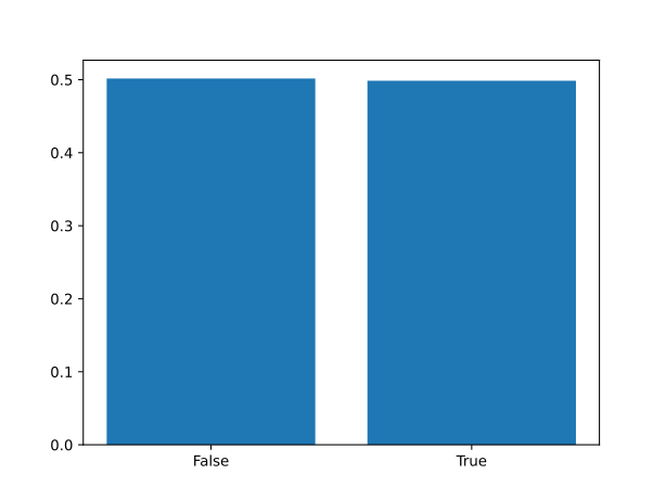
edge _ _ _ = Falser=0.5 and the geometric graph with theta=pi/2. We do this by putting a prior of 0.5 on the graph either being Erdős-Rényi or geometric, and then including the observation that there is an edge between two nodes. In this example we do not consider noise: we observe that there definitely is an edge.
exampleB = do
     -- Prior on the type of graph
     b <- sample $ bernoulli 0.5
     let p = if b then Left (erdosRenyi 0.5) else Right (SG 2 (pi / 2))
     -- Randomly sample two vertices and ask whether there is an edge
     c <- sample $ do {a <- new p ; b <- new p ; return $ edge p a b}
     -- Observation that there is in fact an edge
     if c then score 1 else score 0
     return b
(In a Metropolis-Hastings simulation, score 0 has the effect of rejecting that run of the program.)
Metropolis Hastings call.
testB = do
      bws <- mh 1 $ exampleB
      plotHistogram "graph-edge.svg" $ map fst $ take 100000 bws
Geometric graph inference
Ready.
- 95% predictive interval
- log-likelihood low high
- Observations
Numerical results
Scroll within the table for more values.
Ready.
- log-likelihood low high
- Observations
Numerical results
Scroll within the table for more values.
Ready.
- log-likelihood low high
- Observations
Numerical results
Scroll within the table for more values.
Ready.
- Posterior programs (lines)
- Observations
Numerical results
Scroll within the table for more values.
Ready.
- log-likelihood low high
- Observations
Numerical results
Scroll within the table for more values.
exampleC = do
     -- Prior on the type of graph
     b <- sample $ bernoulli 0.5
     let p = if b then Left (erdosRenyi 0.5) else Right (SG 2 (pi / 2))
     -- Randomly sample three vertices and ask whether they form a triangle
     c <- sample $ isTriangle p
     -- Observation that there is a triangle
     if c then score 1 else score 0
     return b
Metropolis Hastings call.
testC = do
      bws <- mh 1 $ exampleC
      plotHistogram "graph-triangle.svg" $ map fst $ take 100000 bws
We see that a triangle is more likely to have come from the geometric graph. 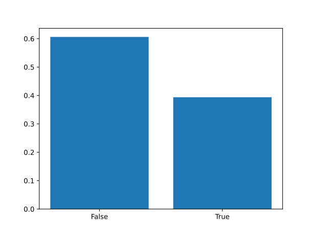
For this particular example we can also do an pen-on-paper calculation to solve the problem, which gives probabilities and respectively, matching this output from the probabilistic programming inference.
Pen-on-paper calculation.
Indeed: Given that the probability of observing a triangle in an Erdős-Rényi graph with is , let’s understand the probability of observing a triangle in a geometric graph on the unit circle.
The probability of having an edge between two points on the unit circle – i.e. the probability that they are at a distance of at most from each other – is . Therefore, since the samples are independent, is the product of
and
By uniformity, the latter probability is the average length (divided by the total circumference of the unit circle) of the arc where the third point can land (expected value of the indicator random variable). This arc can range (linearly) between two extremes:
- When the first two points are as far apart as possible (i.e., there’s a distance of between them): in this case, the third point has to be between the two, in this arc (corresponding to of the circle circumference).
- When the first two points overlap: in this case, the third point can be anywhere around them, i.e., on an arc length of , which is of the circle circumference.
Thus, the probability of observing a triangle in the geometric graph is:
Renormalizing the probabilities from both scenarios, we get, as expected:
- Geometric graph scenario:
- Erdős-Rényi scenario:
Plotting code.
graphToDot :: [[Bool]] -> String
graphToDot g = let vs = [0..length g -1] in
               "graph {node[shape=point] \n edge[len=0.5] \n " ++
               concat [show v ++ "\n" | v <- vs] ++
               concat [show v ++ " -- " ++ show w ++ "\n" | v <- vs , w <- [0..v] , g !! v !! w]
++ "}"plotHistogram :: (Show a , Eq a, Ord a) => String -> [a] -> IO ()
plotHistogram filename xs = do
putStrLn $ "Generating " ++ filename ++ "..."
let categories = sort $ nub xs
let counts = map (\c -> length $ filter (==c) xs) categories
file filename $ bar (map show categories) $ map (\n -> (fromIntegral n)/(fromIntegral $ length xs)) counts
putStrLn $ show $ zip categories $ map (\n -> (fromIntegral n)/(fromIntegral $ length xs)) counts
putStrLn $ "Done."
-- Plot histographs of chances of triangles in different graphs.
testD = do
onER <- mh 1 $ sample $ isTriangle $ erdosRenyi 0.5
onCircle <- mh 1 $ sample $ isTriangle $ SG 2 (pi/2)
onSphere <- mh 1 $ sample $ isTriangle $ SG 3 (pi/2)
onSphereFour <- mh 1 $ sample $ isTriangle $ SG 4 (pi/2)
plotHistogram "tris-ER" $ map fst $ take 10000 onER
plotHistogram "tris-s1" $ map fst $ take 10000 onCircle
plotHistogram "tris-s2" $ map fst $ take 10000 onSphere
plotHistogram "tris-s3" $ map fst $ take 10000 onSphereFour
main = do {showTestData; testA; testB; testC}