Gaussian process regression in LazyPPL
Extensions and imports for this Literate Haskell file
{-# LANGUAGE CPP #-}
module GaussianProcessDemo where
import LazyPPL
import LazyPPL.Distributions (normal, normalLogPdf)
import LazyPPL.Distributions.GP
import Control.Monad
import Numeric.Log (Log(Exp))import Graphics.Matplotlib hiding (density)We can define a random function gp :: (Double -> Double -> Double) -> Prob (Double -> Double) which describes a Gaussian process. This requires an infinite number of random choices, first because it is defined for arbitrarily large x, but also it needs an infinite number of random choices in each finite interval. This is all dealt with using laziness. We cannot plot the function precisely, but when we plot it with a fixed resolution and viewport, it is fine because only finitely many random choices are triggered.
The following defines a GP prior generated with the radial basis function, a.k.a. squared exponential covariance.
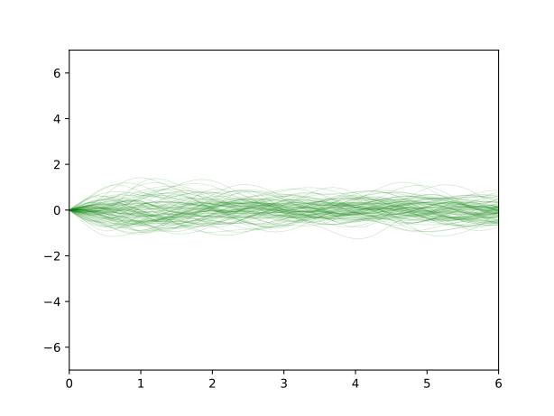
(Plotting code)
rbf var l x1 x2 = var * exp (-(x1 - x2)^2 / (2 * l^2))plotGPPrior =
do
fws <- mh 1 $ sample $ gp $ rbf 0.25 0.5
let xys = map (\f -> map (\x -> (x,f x)) [0,0.1..6]) $ map fst $ take 100 $ fws
plotCoords "images/gp-prior.svg" [] xys (-7) 7 0.2dataset :: [(Double, Double)]
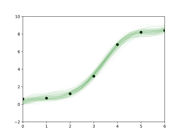
dataset = [(0,0.6), (1, 0.7), (2,1.2), (3,3.2), (4,6.8), (5, 8.2), (6,8.4)]g plus a random start point a. (Note that we are treating this g as a function like any other. And we could also have built this model with the second-order regress function from the other regression examples.)
example :: Meas (Double -> Double)
example = do g <- sample $ gp $ rbf 1 1
             a <- sample $ normal 0 3
             b <- sample $ normal 0 3
             let f x = a + b * x + (g x)
             forM_ dataset (\(x,y) -> scoreLog $ Exp $ normalLogPdf (f x) 0.3 y)
return fplotGPRegression =
do
fws <- mh 0.2 example
let xys = map (\f -> map (\x -> (x,f x)) [0,0.1..6]) $ map fst $ take 100 $ every 1000 $ drop 10000 $ fws
plotCoords "images/gp-reg.svg" dataset xys (-2) 10 0.1Gaussian-process regression
Ready.
- 95% predictive interval
- log-likelihood low high
- Observations
Numerical results
Scroll within the table for more values.
Ready.
- log-likelihood low high
- Observations
Numerical results
Scroll within the table for more values.
Ready.
- log-likelihood low high
- Observations
Numerical results
Scroll within the table for more values.
Ready.
- Posterior programs (lines)
- Observations
Numerical results
Scroll within the table for more values.
Ready.
- log-likelihood low high
- Observations
Numerical results
Scroll within the table for more values.
Graphing routines
plotCoords :: String -> [(Double,Double)] -> [[(Double,Double)]] -> Double -> Double -> Double -> IO ()
plotCoords filename dataset xyss ymin ymax alpha =
    do  putStrLn $ "Plotting " ++ filename ++ "..."
        file filename $ foldl (\a xys -> a % plot (map fst xys) (map snd xys) @@ [o1 "go-", o2 "linewidth" (0.5 :: Double), o2 "alpha" alpha, o2 "ms" (0 :: Int)]) (scatter (map fst dataset) (map snd dataset) @@ [o2 "c" "black"] % xlim (0 :: Int) (6 :: Int) % ylim ymin ymax) xyss
        putStrLn "Done."
        return ()

main :: IO ()
main = do { plotGPPrior ; plotGPRegression }