Linear and piecewise linear regression with LazyPPL
We discuss Bayesian linear regression and piecewise linear regression. Our piecewise linear regression uses an infinite Poisson process as the set of change points. The laziness of Haskell effectively truncates the infinite process as needed. The examples also demonstrate that higher-order functions (such as regress and splice) are very useful.
Extensions and imports for this Literate Haskell file
{-# LANGUAGE CPP #-}
module RegressionDemo where
import LazyPPL
import LazyPPL.Distributions
import Control.Monad
import Numeric.Log (Log(Exp))import Graphics.Matplotlib hiding (density)Linear regression
Regression is about finding a fitting function to some data. Bayesian regression is about finding a posterior distribution on functions, given the data.
We start with a random linear function:
linear :: Prob (Double -> Double)
linear =
  do
    a <- normal 0 3
    b <- normal 0 3
    let f = \x -> a * x + b
    return f
Note that this returns a random function. Here are 1000 draws from the distribution. 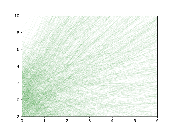
(Plotting code)
plotLinearPrior =
  do
    fs' <- mh 1 (sample linear)
    let fs = map fst $ take 1000 $ fs'
plotFuns "images/regression-linear-prior.svg" [] fs 0.1dataset :: [(Double, Double)]
dataset = [(0,0.6), (1, 0.7), (2,1.2), (3,3.2), (4,6.8), (5, 8.2), (6,8.4)]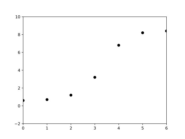
(Plotting code)
plotDataset =
  do
    plotFuns "images/regression-dataset.svg" dataset [] 0.1
Our regression here is noisy: the function has not precisely generated this data set, because the points are not colinear.
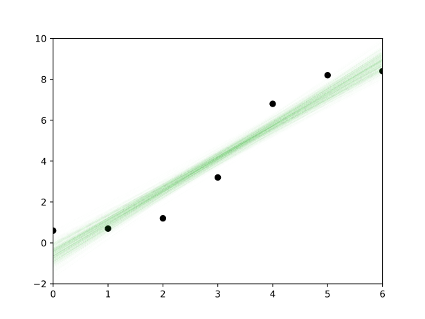
Our generic regression function takes a random functionprior, and some input/output observations dataset, which are assumed to be noisy according to sigma, returns a conditioned random linear function (unnormalized).
regress :: Double -> Prob (a -> Double) -> [(a, Double)] -> Meas (a -> Double)
regress sigma prior dataset =
  do
    f <- sample prior
    forM_ dataset (\(x, y) -> scoreLog $ Exp $ normalLogPdf (f x) sigma y)
return fplotLinReg =
do fs' <- mh 0.5 (regress 0.5 linear dataset)
let fs = map fst $ take 1000 $ every 50 $ drop 100 fs'
plotFuns "images/regression-linear-reg.svg" dataset fs 0.01Bayesian linear regression
Ready.
- 95% predictive interval
- log-likelihood low high
- Observations
Numerical results
Scroll within the table for more values.
Ready.
- log-likelihood low high
- Observations
Numerical results
Scroll within the table for more values.
Ready.
- log-likelihood low high
- Observations
Numerical results
Scroll within the table for more values.
Ready.
- Posterior programs (lines)
- Observations
Numerical results
Scroll within the table for more values.
Ready.
- log-likelihood low high
- Observations
Numerical results
Scroll within the table for more values.
Piecewise linear regression and Poisson point processes
To move to piecewise linear regression, we introduce a functionsplice which splices together different draws from a random function at a random selection of change points. NB if the point process is infinite then the resulting function has an infinite number of pieces, but this is all done lazily, so it’s not a problem.
splice :: Prob [Double] -> Prob (Double -> Double) -> Prob (Double -> Double)
splice pointProcess randomFun =
  do
    xs <- pointProcess
    fs <- mapM (const randomFun) xs
    default_f <- randomFun
    let h :: [(Double, Double -> Double)] -> Double -> Double
        h [] x = default_f x
        h ((a, f) : xfs) x | x <= a = f x
        h ((a, f) : xfs) x | x > a = h xfs x
return (h (zip xs fs))linear, and for a point process we will use the following Poisson point process, poissonPP. This generates an infinite random list of points, where the gaps between them are exponentially distributed.
poissonPP :: Double -> Double -> Prob [Double]
poissonPP lower rate =
  do
    step <- exponential rate
    let x = lower + step
    xs <- poissonPP x rate
    return (x : xs)
Here are five draws from the process. Each draw is really an infinite set of points, but we have truncated the display to the viewport [0,20]. Laziness then takes care of truncating the infinite sequences appropriately. 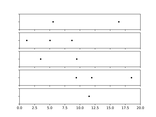
(Plotting code)
plotPoissonPP =
  do
    pws <- mh 1 $ sample $ poissonPP 0 0.1
    let ps = map (takeWhile (20>)) $ map fst $ take 5 $ pws
    let filename = "images/regression-poissonpp.svg"
    putStrLn $ "Plotting " ++ filename ++ "..."
    let myscatter mpl i = mpl % setSubplot i % scatter (ps !! i) (map (const (0::Double)) (ps !! i)) @@ [o2 "s" (10::Int),o2 "c" "black"]  % xlim (0::Int) (20::Int) % ylim (-1 :: Int) (1::Int) % mp # "ax.yaxis.set_major_formatter(mticker.NullFormatter())"
    let myscatteraxes mpl i = if i < (length ps - 1) then myscatter mpl i % mp # "ax.xaxis.set_major_formatter(mticker.NullFormatter())" else myscatter mpl i
    file filename $ foldl myscatteraxes (subplots @@ [o2 "nrows" (length ps),o2 "ncols" (1::Int)]) [0..(length ps - 1)]
    putStrLn $ "Done."
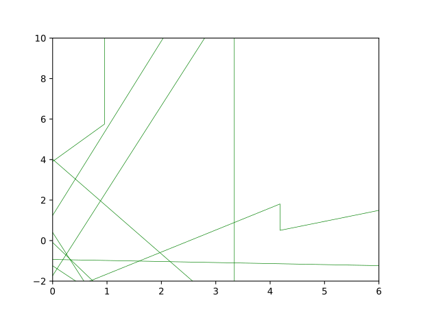
We can now invoke a random piecewise linear function by calling splice (poissonPP 0 0.1) linear. Here are ten draws from this distribution. Because the viewport is bounded, laziness takes care of truncations to the point process that we passed to splice.
(Plotting code)
plotPiecewisePrior =
  do
    fs' <- mh 1 $ sample $ splice (poissonPP 0 0.1) linear
    let fs = map fst $ take 10 $ fs'
plotFuns "images/regression-piecewise-prior.svg" [] fs 1regress 0.1 (splice (poissonPP 0 0.1) linear). We can then sample from the unnormalized distribution using Metropolis-Hastings.
plotPiecewiseReg =
  do
    fs' <- mhirreducible 0.2 0.1 (regress 0.1 (splice (poissonPP 0 0.1) linear) dataset)
    let fs = map fst $ take 1000 $ every 1000 $ drop 10000 fs'
    plotFuns "images/regression-piecewise-reg.svg" dataset fs 0.01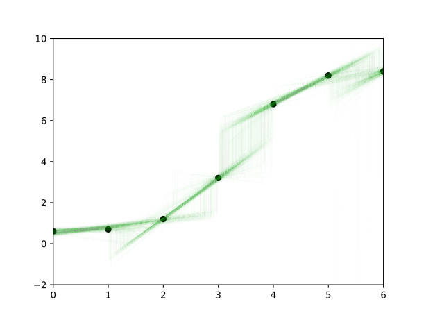
randConst, a random linear function with slope 0.
randConst :: Prob (Double -> Double)
randConst =
  do
    b <- normal 0 3
    let f = \x -> b
return fsplice (poissonPP 0 0.1) randConst and perform inference on it to get the resultant unnormalized distribution of piecewise constant functions.
plotPiecewiseConst =
  do
    fs' <- mhirreducible 0.2 0.1 (regress 0.1 (splice (poissonPP 0 0.1) randConst) dataset)
    let fs = map fst $ take 1000 $ every 1000 $ drop 10000 fs'
    plotFuns "images/regression-piecewise-const.svg" dataset fs 0.01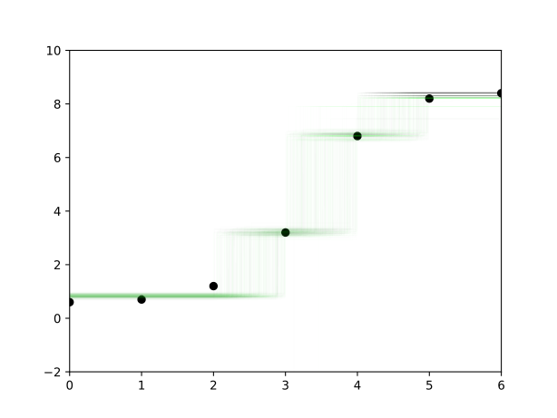
Graphing routines
-- Plot the points drawn from weighted samples
-- epsilon: smallest y axis difference to worry about
-- delta: smallest x axis difference to worry aboutinterestingPoints :: (Double -> Double) -> Double -> Double -> Double -> Double -> [Double] -> [Double]
interestingPoints f lower upper epsilon delta acc =
if abs(upper - lower) < delta then acc
else
let mid = (upper - lower) / 2 + lower in
if abs((f(upper) - f(lower)) / 2 + f(lower) - f(mid)) < epsilon
then acc
else interestingPoints f lower mid epsilon delta (mid : (interestingPoints f mid upper epsilon delta acc))
sampleFun f =
-- [ (x, f x) | x <- [(-0.25),(-0.25+0.1)..6.2]]
let xs = ((-0.25) : (interestingPoints f (-0.25) 6.2 0.3 0.001 [6.2])) in
map (\x -> (x,f x)) xs
plotFuns :: String -> [(Double,Double)] -> [Double -> Double] -> Double -> IO ()
plotFuns filename dataset funs alpha =
do putStrLn $ "Plotting " ++ filename ++ "..."
file filename $ foldl (\a f -> let xfs = sampleFun f in a % plot (map fst xfs) (map snd xfs) @@ [o1 "go-", o2 "linewidth" (0.5 :: Double), o2 "alpha" alpha, o2 "ms" (0 :: Int)]) (scatter (map fst dataset) (map snd dataset) @@ [o2 "c" "black"] % xlim (0 :: Int) (6 :: Int) % ylim (-2 :: Int) (10 :: Int)) funs
putStrLn "Done."
return ()
main :: IO ()
main = do {plotLinearPrior ; plotDataset ; plotLinReg ; plotPiecewisePrior ; plotPoissonPP ; plotPiecewiseReg ; plotPiecewiseConst }