Feature finding using an Indian Buffet Process

A demonstration of using Indian Buffet Process for feature finding. Following A Nonparametric Bayesian Method for Inferring Features From Similarity Judgments. Navarro and Griffiths. NeurIPS 2006.

Extensions and imports for this Literate Haskell file

Haskell

{-# LANGUAGE CPP #-}
{-# LANGUAGE ScopedTypeVariables #-}

Haskell

module AdditiveClusteringDemo where

Haskell

import LazyPPL
import LazyPPL.Distributions
import LazyPPL.Distributions.IBP
import LazyPPL.Distributions.Memoization

Haskell

import Data.List
import Control.Monad
import Data.Monoid

Haskell

import Data.Array
import Data.Maybe

Haskell

import Graphics.Matplotlib
import Helpers (featureMembership, featureRowTicks, featureShade)

Additive clustering is a method for inferring features over a set of of objects using similarity data. The nature of the features is unknown, and the number of possible features is unknown, and inferred using the Indian Buffet Process. Each feature has an associated “saliency” weight indicating how much it contributes to the similarity coefficient. We also infer the saliency weights.

Data set

Haskell

data Country = China | Cuba | Germany | Indonesia | Iraq | Italy | Jamaica | Japan | Libya | Nigeria | Philippines | Russia | Spain | US | Vietnam | Zimbabwe deriving (Eq, Ord, Show, Enum, Bounded, Ix)

Haskell

countries :: [Country]
countries = [China .. Zimbabwe]

Haskell

similarityData :: Array (Country,Country) Double

Data from experiment

Haskell

similarityData = array ((minBound,minBound),(maxBound,maxBound)) [((i,j),if i > j then (countriesDataset !! (fromEnum i) !! (fromEnum j)) else if i == j then 1 else (countriesDataset !! (fromEnum j) !! (fromEnum i))) | i <- countries , j <- countries]
 where
 countriesDataset :: [[Double]] =
  [[ ],
  [0.11],
  [0.06, 0.04],
  [0.43, 0.06, 0.03],
  [0.06, 0.32, 0.04, 0.14],
  [0.02, 0.09, 0.70, 0.02, 0.03],
  [0.02, 0.59, 0.02, 0.14, 0.04, 0.10],
  [0.69, 0.01, 0.26, 0.35, 0.03, 0.06, 0.03],
  [0.03, 0.32, 0.01, 0.04, 0.70, 0.04, 0.11, 0.01],
  [0.01, 0.12, 0.01, 0.04, 0.20, 0.03, 0.31, 0.01, 0.45],
  [0.42, 0.12, 0.01, 0.87, 0.09, 0.02, 0.17, 0.31, 0.05, 0.04],
  [0.51, 0.35, 0.55, 0.01, 0.13, 0.22, 0.02, 0.17, 0.05, 0.02, 0.03],
  [0.02, 0.37, 0.58, 0.03, 0.04, 0.90, 0.20, 0.04, 0.04, 0.03, 0.04, 0.15],
  [0.30, 0.11, 0.42, 0.03, 0.06, 0.20, 0.12, 0.46, 0.02, 0.04, 0.01, 0.43, 0.20],
  [0.60, 0.12, 0.03, 0.55, 0.12, 0.01, 0.05, 0.45, 0.10, 0.03, 0.57, 0.08, 0.02, 0.12],
  [0.01, 0.08, 0.01, 0.11, 0.15, 0.02, 0.29, 0.01, 0.31, 0.83, 0.08, 0.01, 0.02, 0.01, 0.03]]

Data set taken from Representing Stimulus Similarity, PhD thesis, D. J. Navarro. Department of Psychology University of Adelaide. December, 2002

Additive clustering model

The Indian Buffet Process provides abstract types Restaurant and Dish, and the following interface:

newRestaurant :: Double -> Prob Restaurant opens a new restaurant;
newCustomer :: Restaurant -> Prob [Dish] assigns a finite set of dishes to a new customer.

Our additive clustering models has three parameters (alpha, lambda1 and lambda2) and produces a mapping from countries to lists of features. We use an Indian Buffet Process abstraction, so we imagine that each country arrives as a customer at a buffet, and takes some dishes, which are the features. We can then assess which countries took similar dishes to see which countries are similar.

Haskell

additiveClustering :: Double -> Double -> Double
                   -> Array (Country,Country) Double -> Meas (Array Country [Dish])

(Recall that in Haskell, the type (Array a b) comprises a-indexed arrays of things of type b.)

Haskell

additiveClustering alpha lambda1 lambda2 similarityData = do
    (restaurant :: Restaurant) <- sample $ newRestaurant alpha

Each dish is randomly assigned a weight, which is how important it is to the similarities between countries.

Haskell

    (weights :: Dish -> Double) <- sample $ memoize (\d -> gamma lambda1 lambda2)

Each country is assigned a list of dishes, by regarding it as a new customer in the restaurant.

Haskell

    (features :: Array Country [Dish])
           <- listArray (minBound,maxBound) <$>
              (replicateM (fromEnum (maxBound :: Country) + 1) $
              sample $ newCustomer restaurant)

We define a function that calculates the similarity of two countries given the dishes that they share.

Haskell

    let similarity :: Country -> Country -> Double
        similarity i j = sum [weights a | a <- features!j, a `elem` features!i]

We score based on how closely this similarity matches the experimental data.

Haskell

    mapM_ (\(i, j) -> score $ normalPdf (similarityData!(i,j)) 0.1 (similarity i j)) [ (i, j) | i <- countries, j <- countries, j < i ]

We return the feature assignment.

Haskell

    return features

Simulation

We sample from this using Metropolis Hastings simulation, and plot the features of the sample with the highest likelihood. The columns represent the found features, with a coloured box if the country has that feature.

Haskell

test = do
  samples <- mhirreducible 0.2 0.01 $ additiveClustering 2 6 0.3 similarityData
  return $ plotFeatureMatrix $ maxap $ take 100000 samples

Indian buffet process: feature finding

Random seed

Ready.

Numerical results

Observation noise

Ready.

95% predictive interval
log-likelihood low high
Observations

Numerical results

Posterior functions

Ready.

log-likelihood low high
Observations

Numerical results

Posterior functions

Ready.

log-likelihood low high
Observations

Numerical results

Inference steps

Ready.

Numerical results

Inference steps

Ready.

Numerical results

Posterior programs

Ready.

Posterior programs (lines)
Observations

Numerical results

Inference steps

Ready.

Numerical results

Inference steps

Ready.

Numerical results

Lifetime

Ready.

Numerical results

Posterior functions

Ready.

log-likelihood low high
Observations

Numerical results

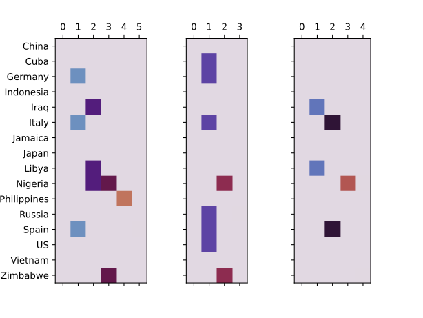
This is a highly multi-modal distribution. For the three runs, we typically have different numbers of features, and they are different. But in each case they admit a human interpretation, for example geographic, history, development status.

Plotting routines

Haskell

-- The sample with the highest weight, that is, the highest likelihood
maxap samples =
        let maxw = (maximum $ map snd samples) in
        fromJust $ Data.List.lookup maxw $ map (\(z,w) -> (w,z)) samples

Haskell

plotFeatureMatrix :: (Ix x,Show x,Eq y) => Array x [y] -> Matplotlib
plotFeatureMatrix features = do
  let matrix = featureMembership features
      columns = maximum (0 : map length matrix)
      ticks = featureRowTicks features
  matShow (map (map (featureShade columns)) matrix) @@ [o2 "cmap" $ raw "twilight", o2 "vmin" (0 :: Double), o2 "vmax" (1 :: Double)] % yticks (map fst ticks) % ytickLabels (map (raw . show . snd) ticks)

Haskell

combinePlots filename fs = do
  putStrLn $ "Generating " ++ filename ++ "..."
  file filename $ foldl (\p i -> p % setSubplot i % fs !! i) (subplots @@ [o2 "ncols" (length fs), o2 "sharey" True, o2 "gridspec_kw" $ lit "{'width_ratios': [1, 1, 1]}"]) [0..(length fs -1)]
  putStrLn "Done."

Haskell

main = do { ps <- replicateM 3 test ; combinePlots "images/additiveclustering-matrix.svg" ps }